An introduction to Gradient Boosting Machine

In this Saturday morning, I decide to have a look through an ensemble method that has recently driven many successes on Kaggle competitions called “Gradient Boosting Machine”. I then try to reimplement it in python so that I can understand it better in practice.

As its name indicates, GBM trains many models turn by turn and each new model gradually minimises the loss function of the whole system using Gradient Descent method. Assuming each individual model i is a function h(X;pi)(which we call “base function” or “base learner”) where X is the input and pi is the model parameter. Now let’s choose a loss function L(y,y′) where y is the training output, y′ is the output from the model. In GBM, y′=∑Mi=1βih(X;pi) where M is the number of base learners. What we need to do now is to find:

β,P=argmin{βi,pi}M1L(y,∑i=1Mβih(X;pi))

However this is not easy to achieve optimal parameters. Instead we can try a greedy approach that reduces the loss function stage-by-stage:

βm,pm=argminβ,pL(y,Fm−1(X)+βh(X;p))

And then we update:

Fm=Fm−1(X)+βmh(X;pm)

In order to reduce L(y,Fm), an obvious way is to step toward the direction where the gradient of L descents:

−gm(X)=–[∂L(y,F(X))∂F(X)]F(X)=Fm−1(X)

However what we want to find out is βm and pm so that Fm∼Fm−1–gm. In another way, βmh(X;pm) is most similar to −gm:

βm,pm=argminβ,p∑i=1N[−gm(xi)–βh(xi;p)]2

We can then fine-tune βm so that:

βm=argminβ′L(y,Fm−1(X+β′h(x;p)))

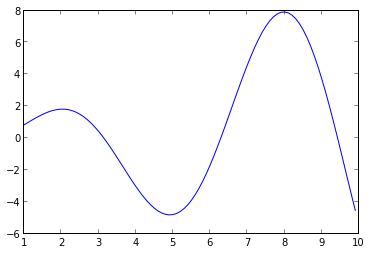
I wrote a small python script to demonstrate a simple GBM trainer to learn y=xsin(x) over the base function y=xexp(x) using the loss function L(y,y′)=∑i(yi–y′i)2:

1 2 3 4 5 6 7 8 9 10 11 12 13 14 15 16 17 18 19 20 21 22 23 24 25 26 27

from numpy import * from matplotlib import * from scipy.optimize import minimize def gbm(L, dL, p0, M=10):     """ Train an ensemble of M base leaners.     @param L: callable loss function     @param dL: callable loss derivative     @param p0: initial guess of parameters     @param M: number of base learners     """     p = minimize(lambda p: square(-dL(0) - p[0]*h(p[1:])).sum(), p0).x     F = p[0]*h(p[1:])     Fs, P, losses = [array(F)], [p], [L(F)]     for i in xrange(M):         p = minimize(lambda p: square(-dL(F) - p[0]*h(p[1:])).sum(), p0).x         p[0] = minimize(lambda a: L(F + a*h(p[1:])), p[0]).x         F += p[0]*h(p[1:])         Fs.append(array(F))         P.append(p)         losses.append(L(F))     return F, Fs, P, losses X = arange(1, 10, .1) Y = X*sin(X) plot(X, Y)

1 2 3 4 5 6 7 8 9 10

h = lambda a: a[0]*exp(a[1]*X) L = lambda F: square(Y - F).sum() dL = lambda F: F - Y a0 = asarray([1, 1, 1]) # Build an ensemble of 100 base leaners F, Fs, P, losses = gbm(L, dL, a0, M=100) f = figure(figsize=(10, 10)) _ = plot(X, Y) _ = plot(X, zip(*Fs))

1 2	#plot losses after each base leaner is added plot(losses)

At the end, I would like to recommend Scikit learn to you – a great Python library to work with GBM.

Bibliography
Friedman H J. Greedy Function Approximation: A Gradient Boosting Machine. IMS 1999 Reitz Lecture. URL:http://www-stat.stanford.edu/~jhf/ftp/trebst.pdf.